GIS II Final Project: GIS Application in Conservation Biology

Goals and Objectives

The basis of this study is to understand more about the distribution and habitat of the Oregon spotted frog in order to find areas to protect this species while taking outside factors into account. I chose this study in order to provide an example of GIS application in conservation biology. Using the GIS data to examine where the species are found and what the nearest threats to their habitats are will allow for new protection plans to be developed.

Background

The Oregon Spotted frog is found only in the Northwestern United States and Canada, in lentic freshwater habitats and wetlands (McAllister & Leonard 1997). The species’ habitat is threatened by residential development, dam construction, and grazing by other animals. Habitat degradation is the greatest threat to this species and data shows how drastically the range of the Oregon spotted frog has decreased over the years (McAllister & Leonard 1997). Other threats include introduced fish predators and bullfrogs. It is currently listed on the IUCN red list as Vulnerable, and it is a candidate for listing in the US Endangered Species Act (The IUCN Red List of Endangered Species). There are no major conservation actions being taken to protect this species, however the US Fish and Wildlife service has a Sensitive Species policy which requires the agency to maintain and preserve the populations of all native species in habitats on National Forest lands (Cushman & Pearl 2007).

Methods

Project all feature classes to NAD 1983, because that is the GCS that the California Oregon Spotted Frog data was projected in and this makes it easier

Create study area of these 4 counties: Siskiyou county, Modoc county, Shasta county, and Lassen county because these are the four counties in which the Oregon Spotted Frog has been recorded. Select by attributes to select the 4 counties, create layer from selection. Rename it Study Area

Convert raster to polygon feature based on the LIFE_FORM field, which defines the type of life form the frog is found on in that area. Categories are: Conifer, Hardwood, Herbaceous, Shrub, and Water. This information is useful because it shows what type of life forms the frogs prefer and therefore the most important ones to protect.

Calculate statistics on Shape_Area Sum to discover the top three Results: the frog appears to prefer conifer, herbaceous plants, and water the most.

Clip major roads from Usa data from UWEC geog dept. to the study area.

Clip CA_Lakes feature class to study area

Buffer 0.5 miles around roads due to future construction highly likely in those areas, therefore it is not realistic to restrict construction in these areas. Use ModelBuilder to execute this tool.
Buffer 1, 3, and 5 miles around the range for potential protection areas
Use edit tools to reshape the 5 mile buffer area to avoid roads

Results

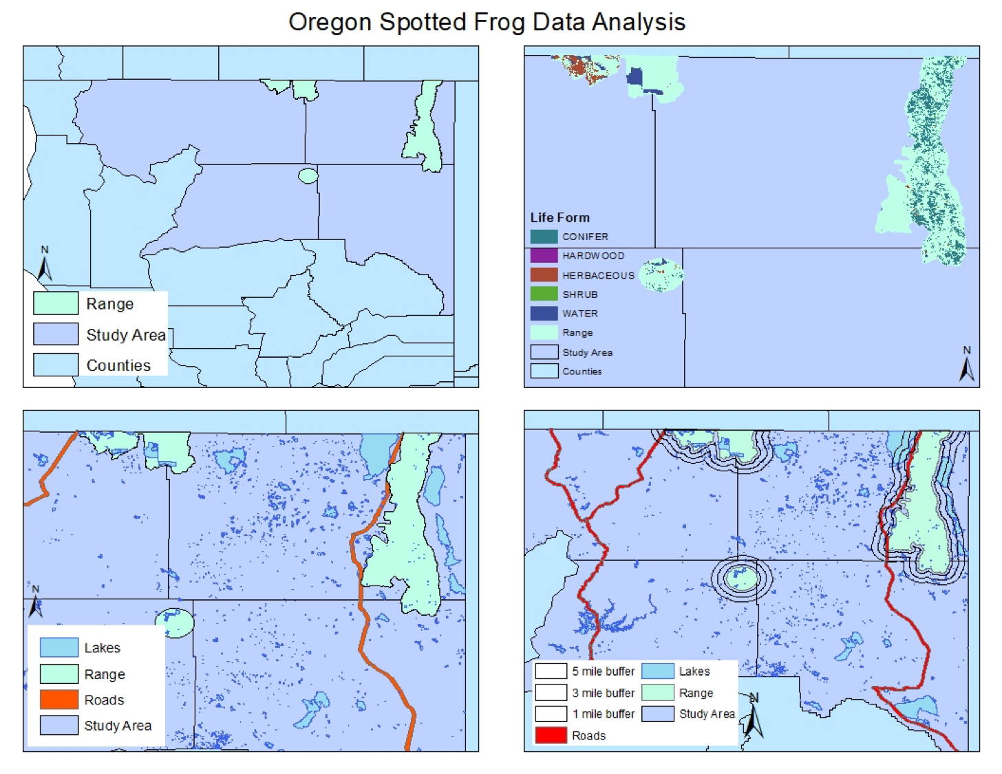Figure 1. Top left image shows range map of the OSF in the study area of the four counties in N. California. Top right shows the types of life forms that the frogs were found on or near, Bottom left shows added lakes and roads, and bottom right shows the added 1, 3, and 5 mile buffers.

Figure 2. Resulting map image with green areas representing potential OSF reserves

I settled on just reshaping the 5-mile range buffer to avoid the major roads. This is definitely not what a professional would have done because this project truly requires far more research, but this is a nice start to showing how GIS is generally used in conservation biology

Conclusions
Throughout this project I learned that these things really take an immense amount of planning. Model Builder was very helpful for the tedious tools that I had to apply multiple times. I also learned that finding areas for environmental protection is a lot more complicated and involves many factors beyond the ones that I explored in this study. Opportunity for further analysis could include residential developments as well as commercial development. Further analysis of habitat and microclimate could also be considered. I gained some experience of using GIS for biological application and now understand how much more complex these projects are.

Sources
Cushman, Kathleen A, and Christopher A Pearl. “A Conservation Assessment for...” USDI Bureau of Land Management, Mar. 2007.

Drapera, D. A.-G. Application of GIS in plant conservation programmes in Portugal. Biological Conservation. 2003. 

McAllister, Kelly R, and William P Leonard. “Oregon Spotted Frog.” Washington State Status Report. Wash. Dept. Fish and Wild., Olympia. July 1997.

Shah, Anup. “Why Is Biodiversity Important? Who Cares?.” Global Issues. 19 Jan. 2014. Web. 29 Oct. 2017.

“Species Profile for Oregon Spotted Frog (Rana Pretiosa).” Environmental Conservation Online System, US Fish and Wildlife Service.

The IUCN Red List of Threatened Species. Version 2017-2

Datasets acquired from the California Department of Fish and Wildlife geoportal and ArcGIS online.

GIS II Lab 3: Geodatabase development

Goals
The goal of this lab exercise is to create documentation of the organization and planning for a personal project geodatabase schema. The components and behavior of the geodatabase will also be developed and outlined in this lab.

Methods
Part 1: Developing the geodatabase schema
To develop a geodatabase schema, these questions must be considered:
What is the vision and purpose? The purpose of the project is to identify areas suggested for protecting the sensitive species, Oregon Spotted Frog in Northern California. The geodatabase will provide a place to store all of the necessary shapefiles and models to be worked with.
Who may use it and why? I will be the only one to use it since it is a personal course project, however my professor may have access to it.
Which type did you choose? I chose the File Geodatabase because a Personal Geodatabase only allows 2GB of storage, and I may need more than that. If this were a project being done for the government, I would use an Enterprise Geodatabase so that multiple people could work with the data and edit simultaneously.
What are the geographic characteristics? (area extent, map scale, projection) The map projection will be NAD 1983. All layers that were not previously in NAD 1983 will be reprojected. The map scale will be 1:100,000 to show the area of Northern California where the frog is typically found. The area extent will be from the west coast of California to the eastern border, and from the northern border down to San Francisco.
Did you incorporate topology? How about annotations? Why or why not? Topology and annotations will not be necessary. Topology would be used in the future for actually delineating an area for protection, but this project is just to provides suggestions. Annotations will not be used as there should not be any need for them. Simple labels can be used if necessary.
Do you have a plan for metadata? If so, what is it? If not, why not? Much of the original metadata has been provided with the datasets downloaded from Esri Online and the CWHR, and additional processing changes performed by me will be added. 

To create a geodatabase, open ArcCatalog and go to the desired folder in which you'd like to store the geodatabase. Right-click on it and select New > File Geodatabase from the drop down menu. You may then create new feature datasets, feature classes, etc or import feature classes and datasets from other geodatabases.


Part 2: Describing the components and their behavior
Once the schema has been developed, the next step is to define the components and behavior of the geodatabase. This means to describe which datasets are included and why, and then to describe the attribute fields and their content.

1. A polygon feature class showing the range of the Oregon Spotted Frog in California will be used to identify the areas which need to be protected. This layer contains the attributes Sname (Species Name), CName (the common name).
2. A raster file will be converted to polygons using the WHRNAME field which represents the type of habitat, and used to examine the types of habitat within the species range. It will also be used to create a polygon layer with a habitat suitability ranking. A habitat suitability rank of Low, Medium, and High based on expert opinion suitability value us used to identify the best habitats for the species and therefore the most important to be protected.
3. The counties feature class from the mgisdata folder provided by UWEC will be used to create a study area polygon shapefile by clipping the feature class to the four adjacent counties in which the Oregon Spotted Frog is found. The only important attribute field is the county names, used to make a selection for clipping.
4. Infrastructure layers from ArcGIS online will be reprojected and used to identify the places it may be most difficult to ban construction to protect the species.

To outline the behavior settings of the feature classes, include subtypes, coded and/range domains, split and merge policies, and default values that will be utilized. This can be organized into a table like so:

Figure 1. Domain table for the geodatabase

Results

Figure 2. The geodatabase created

Sources
Esri Online
UWEC Department of Geography
California Department of Resources data catalog