The objectives of this lab are to practice and understand the processes involved in delineating watersheds, demonstrate real world applications of watershed analysis, and to gain experience using ModelBuilder for structuring workflows.
Background
Part 1: A watershed is a point at which the surface waters in an area converge. They are important environmental units because if one becomes polluted, the entire area downstream of that becomes polluted as well. Delineating watersheds is important for monitoring the amount and quality of water entering a point of interest. Adirondack Park is the largest protected area in the contiguous United States and has a variety of uses, making it important to understand the sources and flow of water in the area.
Part 2: Denmark has been experiencing detrimental flood damage due to sudden extreme rainfall from cloudbursts. This led the Danish government to develop a Task Force on Climate Change Adaptation. The task force created a map identifying low-lying areas, or "bluespots", that do not have natural drainage. These are areas most susceptible to flooding after a cloudburst. The map is called a bluest map, and this lab demonstrates how to create one.
Methods
Part 1: Delineation of watersheds
To begin this lesson, create a geodatabase to store and process output data. Download the Adirondack park boundary layer from the New York State GIS Clearinghouse. Click on Data > Data Catalog > List datasets by data set name and search for Adirondack Park Boundary. Click Data set details to download and extract the data. Next, download hydrology from the Cornell University Geospatial Information Repository website. Click map browse > statewide data and search Hydrography Features of New York State shapefile from NatlAtlas. Click download now and extract the data.
Lesson 2: Process data
Open ArcMap and check the map projections for the newly obtained data. Use the park boundary shape file's projection for the map (UTM Zone 18N). In ArcToolbox, go to Analysis tools > Proximity > Buffer to add a 20km buffer to the park boundary and set to Dissolve to All. Next, go to Data management Tools > Projections and Transformations > Project and import the projection from the park boundary. Name the output hydro_utm83. Clip the streams layer in hydro_utm83 to the park boundary and save the output as hydro_utm83c. Now add data from ArcGIS online by searching for DEM North American and selecting the 30 arc-second DEM of North America. When the menu pops up, click Transformations and convert from GCS_WGS_1984 to NAD 1983 and click ok and then close. Clip the DEM to the buffered park boundary, being sure to check the box next to Use input features for clipping geometry. Name the output DEMc. Now remove the ArcGIS online layer. Go to Data management tools > Projections and Transformations > Raster > Project raster. Set the input dataset to DEMc and the output to DEM_utm83. Import the park boundary coordinate system. Select the WGS_1984 to NAD_1983 transformation and choose bilinear for the resampling method with a 60 m output cell size. Remove any non-UTM layers from the data frame.
Lesson 3: Delineate watersheds
To calculate the flow directions for each cell in the DEM, go to Spatial Analyst Tools > Hydrology > Flow Direction. DEM_utm83 should be the input raster and name the output flow direction raster flow_dir. To fill sinks, go to Spatial Analyst Tools > Hydrology > Fill and used em_utm83 as the input and name the output filled. Next you will determine flow directions for the filled DEM with the flow direction tool once again, but this time using filled as the input and flow_dir2 for the output. To determine Flow accumulation, use the Flow Accumulation under the Hydrology tools. Name the output flow_acc and make sure the output data type is set to integer. Invert the color ramp from white to black in the Symbology tab of the properties. Now create a source raster by going to Spatial Analyst Tools > Conditional > Con. Make flow_acc the input conditional raster layer, enter value > 50000 in the expression box, and use 1 as the input true raster value. Name the output net_50k. To assign unique identifiers to each stream reach, go to Spatial Analyst Tools > Hydrology > Stream Link. Set net_50k as the input stream raster and flow_dir2 as the input flow direction raster. Name the output raster source. Now to delineate the watersheds. Go to Spatial Analyst Tools > Hydrology > Watershed, and use flow_dir2 as the input flow direction raster, source as the input raster, and watershed_50k for the output raster. Clip the watershed_50k raster to the park boundary and make sure that the Use Input Features for Clipping Geometry is checked. Add the stream shapefile as blue lines to visually compare watershed boundaries with stream locations. Figure 1 represents the results.
Part 2: Find areas at risk of flooding in a cloudburst
Lesson 1: Explore the cloudburst issue by reading the information on the ArcGIS Lesson
Lesson 2: Work with the project data to explore the municipality of Gentofte.
Download and extract the data from the link in the ArcGIS lesson. Open a blank map in ArcMap and confirm that the version being used is 10.3 or later. Click on Customize > Extensions > check the box for Spatial Analyst and close the window.Open ArcCatalog and connect to the Cloudburst folder. Expand the Cloudburst folder in ArcCatalog. There should be a folder, four geodatabases and four toolboxes. The contents of these items are listed in Fig. 1.
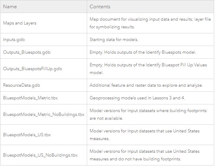 |
| Figure 1. Contents of the Cloudburst folder |
Expand the Maps and Layers folder and open the Gentofte.mxd. In the main menu, select Bookmarks > Study Area to zoom to the study area. Next zoom to the Ordrup bookmark to examine it. Go back to the Study Area bookmark and turn on the DEM layer. Notice that the lighter the shade of brown, the higher the elevation. Now zoom to the Genofte bookmark and use the Identify tool to explore. Change the Identify From setting to DEM and examine the elevations in the lake and surrounding areas.
To explore the DEM metadata, right-click the DEM layer in the Table of Contents > Data > View Item Description. Take note of the resolution. Right click on the DEM layer in the Table of Contents again, but this time select Properties. Click on the Source tab and then scroll down to the Spatial Reference heading. Close the Properties and save the map.
Lesson 3: Find bluespots and affected buildings.
Expand the Cloudburst folder in ArcCatalog and then expand the BluespotModels_Metric toolbox. Right click the Identify Bluespots tool and choose Edit. The ModelBuilder window will appear (Fig. 2). The blue represents input datasets, the yellow represents tools, and the green represents output datasets. Clicking on Windows > Overview will open a small window that denotes which portion of the model is currently visible.
 |
| Figure 2. Identify Bluespots model edit window |
Right click on various tools and inputs and choose "Open.." to examine their parameters. Move the ModelBuilder so that ArcCatalog is visible. Open the Identify Bluespots model and notice that the four parameters correspond to the variables marked with a P in the model. Click cancel and close the tool. At the top of the ModelBuilder window choose Model > Model Properties. Click the Environments tab and the the Values button. Expand the each of the headings to observe them and then close them, keeping the defaults. Close the window.
Now it's time to run the model. Validate the model by clicking the black checkmark button on the ModelBulder toolbar. Once the model is validated, click the sideways blue triangle to run the model. Close the Progress window then the model is finished running. Slick Save on the ModelBuilder window and minimize it. In ArcCatalog, right click the Output_Bluespots.gdb and choose Refresh. Two important datasets have been added, Bluespots and BuildingsTouchBS. Add these to the map in ArcMap and rename BuildingsTouchBS to Buildings Touching Bluespots.
Zoom to the Study Area bookmark. Right-click the Buildings Touching Bluespots later and open attribute table to notice how many buildings are within or adjacent to a bluespot. Close the table. Right-click on the Basemap layer and remove it as well as removing the DEM layer. Turn off the Buildings layer for now. Go to Add Data > Add Basemap and add the Dark Gray Canvas baseman. Close the Geographic Coordinate System warning. Change the symbol for Buildings Touching Bluespots to Yucca Yella color and Outline Width to 0, then click OK. Change the Bluespots layer color to Steel Blue and the Width to 0 as well. Next, change the symbol for the Municipal Boundary layer to the Boundary, City symbol with a color of Gray 10% and width of 1.5. Click OK in all windows. Move the Municipal Boundary layer above the Buildings Touching Bluespots layer in the Table of Contents. Save the map document as Gentofte Bluespots and save the model as well. Close the ModelBuilder window.
Lesson 4: Assess flood risk to buildings
After finding blue spots, this model will calculate their volumes and watersheds to determine the amount of rainfall it takes to fill each bluespot. Open the Gentofte map document and in the Catalog tree, expand the cloudburst folder and BluespotModels__Metric toolbox. Right-click the Identify Bluespot Fill Up Values tool and select edit from the drop-down menu. Observe the functions and then click the Validate Entire Model button. Click Run to run the model once it has been validated. When the model is finished, close the progress window. Save the model and minimize the ModelBuilder window. Open ArcCatalog and expand the Cloudburst folder again. Right-click Outputs_BluespotsFillUp.gdb and refresh. There should be four new feature classes: BSPolyDissolved, BSTouchBuildings, BuildingsTouchBS, and Watersheds. Add the layers BSPolyDissovled, BuildingsTouchBS, and BSTouchBuildings.
To analyze the results, look at the fill-up values for the blue spots and symbolize the ones touching buildings based on those values. Zoom to the Study Area bookmark and open the attribute table for Bluespots Touching Buildings. Sort FillUp in ascending order because the smaller the value, the faster it will fill up therefore the greater the risk. Open the statistics for this field and notice that most of the fill up values are on the low end of the range. Close the statistics and attribute windows. Remove the Basemap, DEM, Buildings, and Bluespots layers from the map. Turn off Buildings Touching Bluespots layer. Add the light gray canvas baseman and ignore the Geographic Coordinate Systems warning. Change the symbol for Municipal Boundary to Gray 60% with a width of 1.5. Open layer properties for Bluespots Touching Buildings and Import from the symbology tab. Browse to Cloudburst > Maps and Layers and add AdjustedFullUpValues.lyr. Click ok. Confirm that Value Field is set to FillUp and click ok again. Notice that the labels for the fill-up values have been adjusted by 40 mm to account for the sewer system capacity. Move the Buildings Touching Bluespots layer above the Bluespots Touching Buildings layer and turn it on. Change the symbol outline width to 0. You now have a Bluespots Fill Up map that can be used for analyzation.
Results
 |
| Figure 3. Delineated watersheds output map |
 |
| Figure 4. Delineated watersheds with a 100,000 source raster threshold yields less watersheds than the 50,000 source raster threshold shown in Fig. 3. |
 |
| Figure 5. Delineated watersheds with a source raster threshold of 500,000 yielding even less watersheds than 50,000 and 100,000 (Fig. 3 & 4) |
 |
| Figure 6. A map representing blue spots in rankings of high risk (low fill-up value) to low risk (high fill-up value) and the buildings located near each. |
 |
| Figure 7. Bluespots and the affected buildings around them in Gentofte, Denmark. |
 |
| Figure 8. The blue spots at the highest risk of flooding based on the lowest fill-up values |
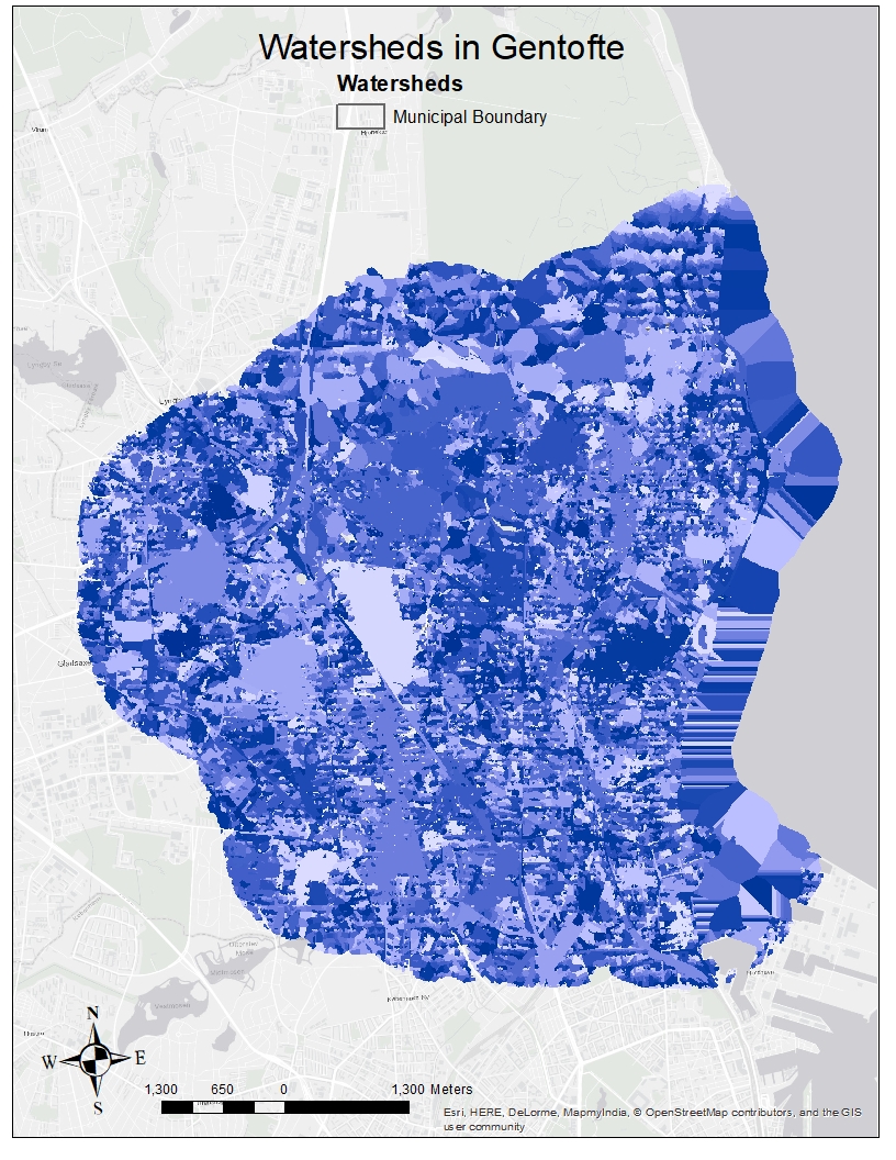 |
| Figure 9. A discrete values map of the watersheds in Gentofte, Denmark. |
 |
| Figure 10. A map representing the roads and railways at least risk of flooding based on their proximity to blue spots with high fill-up values. |
From this lab exercise, an understanding of what watersheds are and how they are useful was gained through the practice of delineated the watersheds in ArcMap and then changing parameters to see how they change the watersheds. The creation of bluespots and additional tools useful for analyzing flood risks were also practiced and helped the user to gain an understanding of the background work that must occur to get to the endpoint where the risk can actually be assessed in the most accurate way.
Sources
The Adirondack Park boundary shapefile was retrieved from the New York State GIS clearinghouse
The hydrology shapefile was retrieved from Cornell University's Geospatial Information Repository (CUGIR)
The 30-second arc DEM was accessed from the ESRI web portal
No comments:
Post a Comment